Scikit-learn-compatible vine-copula estimators

This notebook walks through VineDensity and VineRegressor, the two single-vine estimators that ship with the pyvinecopulib.sklearn extra. Both are thin scikit-learn wrappers around pyvinecopulib.core.Vinecop and pyvinecopulib.utils.Kde1d, providing the standard fit / predict interface plus DataFrame handling, automatic continuous/discrete column inference, and batched evaluation.

All vine copula models are built on Sklar’s theorem, which factorises a joint density into one-dimensional marginals and a copula on the unit hypercube,

\[f(\mathbf{x}) = c\bigl(F_1(x_1), \ldots, F_d(x_d)\bigr) \, \prod_{j=1}^{d} f_j(x_j).\]

The marginals \(F_j\) / \(f_j\) are estimated by univariate KDE (see Kde1d), and the dependence structure \(c\) is decomposed into a tree of bivariate “pair-copulas” — the vine. See the pyvinecopulib.core and pyvinecopulib.families module docs for the underlying machinery; this notebook focuses on the sklearn-facing interface.

Data: the Concrete Compressive Strength dataset from the UCI ML repository (1030 rows, 8 mix-composition features → compressive strength target). The same regression flow is used in the experiments of Vatter & Nagler (2026) — minus the model-confidence-set ensembling, which is the subject of the companion forest notebook.

import time

import matplotlib.pyplot as plt
import numpy as np
import pandas as pd
from sklearn.linear_model import LinearRegression
from sklearn.metrics import mean_absolute_error, root_mean_squared_error
from sklearn.model_selection import train_test_split
from sklearn.preprocessing import StandardScaler

from pyvinecopulib.sklearn import VineDensity, VineRegressor

rng = np.random.default_rng(0)

Data

We load the 1030-row Concrete dataset and standard-scale the covariates. Vines are themselves scale-equivariant (the Kde1d marginal step absorbs any monotone transform), so scaling is purely there to keep the comparison with the linear baseline fair.

# Concrete Compressive Strength dataset from the UCI ML repository.
url = "https://archive.ics.uci.edu/ml/machine-learning-databases/concrete/compressive/Concrete_Data.xls"
df = pd.read_excel(url)
X = df.iloc[:, :-1].values
y = df.iloc[:, -1].values
X_train, X_test, y_train, y_test = train_test_split(
  X, y, test_size=0.2, random_state=42
)
scaler = StandardScaler().fit(X_train)
X_train = scaler.transform(X_train)
X_test = scaler.transform(X_test)
print(f"train: {X_train.shape}, test: {X_test.shape}")

train: (824, 8), test: (206, 8)

Density estimation

VineDensity.fit(X) fits a vine copula to the joint distribution of every column of X. The factorisation from Sklar’s theorem above means the resulting density is a product of seven \(\mathrm{Kde1d}\) marginal densities times a copula density on \([0, 1]^d\) encoding their dependence — and once fitted we can both evaluate it (score_samples, pdf, cdf) and sample from it.

To turn the regression dataset into a generative model we stack the response onto the covariates so VineDensity treats \(Y\) as just another marginal.

joint_train = np.hstack([X_train, y_train.reshape(-1, 1)])
joint_test = np.hstack([X_test, y_test.reshape(-1, 1)])

t0 = time.time()
dens = VineDensity().fit(joint_train)
print(f"VineDensity fit: {time.time() - t0:.1f}s")

nll_test = -float(dens.score_samples(joint_test).mean())
print(f"test NLL: {nll_test:.3f}")
print(
  f"pdf range on test: [{dens.pdf(joint_test).min():.2e}, {dens.pdf(joint_test).max():.2e}]"
)

VineDensity fit: 0.7s
test NLL: 7.199
pdf range on test: [3.22e-11, 1.46e+00]

Sampling

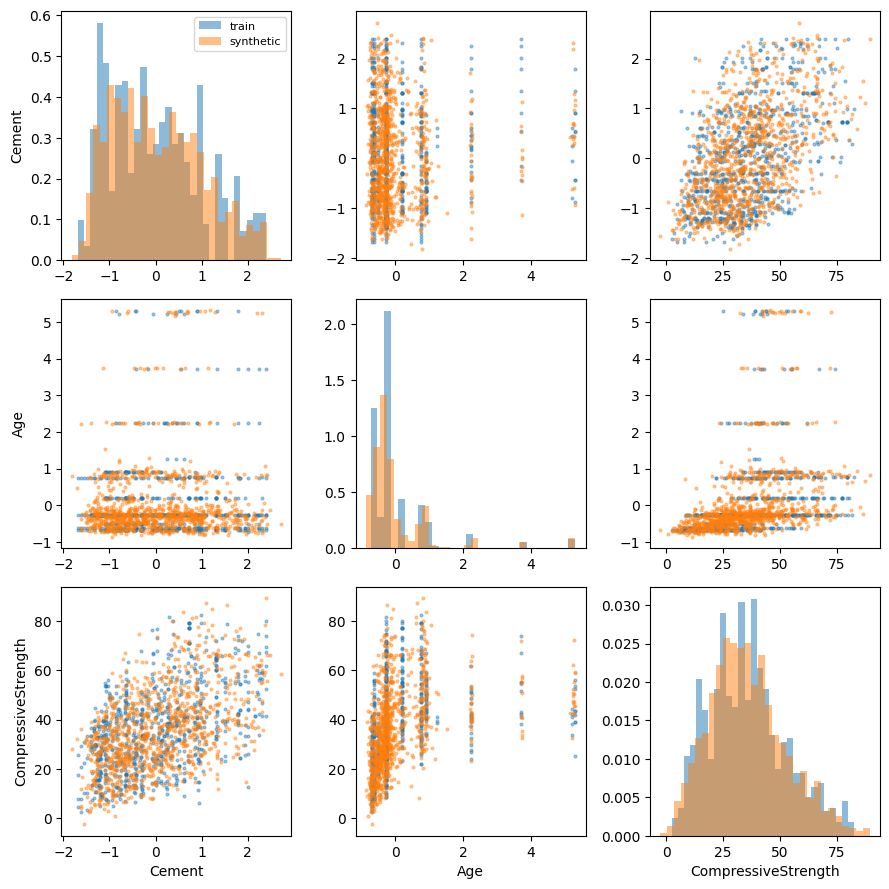
A density estimator that captures dependence should generate synthetic data whose pairwise structure matches the training set. The pair plot below superimposes 1000 draws from dens.sample(...) on the training data for three representative columns (cement content, age, and the response CompressiveStrength). The diagonal panels show marginal histograms; the off-diagonals show scatter plots, which is where dependence is visible.

synth = dens.sample(n_samples=1000, random_state=42)

# Pick three informative columns: Cement (0), Age (7), and the target
# CompressiveStrength (8) on the 8-feature + target joint.
cols_idx = [0, 7, 8]
col_names = ["Cement", "Age", "CompressiveStrength"]
d = len(cols_idx)

fig, axes = plt.subplots(d, d, figsize=(3 * d, 3 * d))
for i in range(d):
  for j in range(d):
    ax = axes[i, j]
    ci, cj = cols_idx[i], cols_idx[j]
    if i == j:
      ax.hist(
        joint_train[:, ci], bins=30, density=True, alpha=0.5, label="train"
      )
      ax.hist(synth[:, ci], bins=30, density=True, alpha=0.5, label="synthetic")
      if i == 0:
        ax.legend(fontsize=8)
    else:
      ax.scatter(
        joint_train[:, cj], joint_train[:, ci], s=4, alpha=0.4, label="train"
      )
      ax.scatter(synth[:, cj], synth[:, ci], s=4, alpha=0.4, label="synthetic")
    if i == d - 1:
      ax.set_xlabel(col_names[j])
    if j == 0:
      ax.set_ylabel(col_names[i])
plt.tight_layout()

Joint CDF

cdf is quasi-Monte-Carlo and so noisy at small N; pass seeds for reproducibility and bump N if the noise floor matters. The joint CDF is small at random points in \(\mathbb{R}^9\) (each marginal contributes a factor \(\le 1\)), so we evaluate at marginal quantiles where the expected monotone behaviour is easier to see.

qs = np.linspace(0.1, 0.9, 5)
# Build points where every coordinate sits at the same marginal quantile.
grid = np.column_stack(
  [np.quantile(joint_train[:, j], qs) for j in range(joint_train.shape[1])]
)
cdf_grid = dens.cdf(grid, N=20000, random_state=0)

print(f"{'marginal quantile':>18}  {'joint CDF':>10}")
for q_lvl, F_val in zip(qs, cdf_grid):
  print(f"{q_lvl:>18.2f}  {F_val:>10.4f}")

 marginal quantile   joint CDF
              0.10      0.0000
              0.30      0.0000
              0.50      0.0001
              0.70      0.0100
              0.90      0.3757

Regression: conditional mean + quantiles

VineRegressor.fit(X, y) fits a vine copula to the joint distribution of \((Y, X)\). Predictions then follow the estimating-equation framework of Nagler & Vatter (2024): for any functional \(\beta(x)\) characterised by \(\mathbb{E}[\psi_\beta(Y) \mid X = x] = 0\), we plug in the fitted conditional density and solve \(\int \psi_\beta(y) \, \hat f(y \mid x) \, dy = 0\). Two standard choices of \(\psi_\beta\) recover familiar predictors,

\[\begin{split}\begin{aligned} \psi_\beta(y) &= y - \beta &&\Rightarrow\; \beta(x) = \mathbb{E}[Y \mid X = x], \\ \psi_\beta(y) &= \mathbf{1}\{y < \beta\} - \tau &&\Rightarrow\; \beta(x) = Q_\tau(Y \mid X = x). \end{aligned}\end{split}\]

Both reduce in practice to a weighted average of the training responses with weights \(w_i(x) \propto c_{Y, X}(\hat F_Y(y_i), \hat F_X(x))\) derived from the fitted copula density — closed-form for the mean, and np.quantile(..., weights=..., method="inverted_cdf") for the conditional quantiles.

predict(X) returns the requested statistics column by column: mean first (when mean=True), then the quantiles in the order configured at construction.

quantiles = np.linspace(
  0.05, 0.95, 19
)  # 5%, 10%, ..., 95% — odd count for CRPS
median_col = 1 + int(np.argmin(np.abs(quantiles - 0.5)))

t0 = time.time()
reg = VineRegressor(mean=True, quantiles=quantiles).fit(X_train, y_train)
print(f"VineRegressor fit: {time.time() - t0:.1f}s")
t0 = time.time()
y_pred = reg.predict(X_test)
print(f"VineRegressor predict: {time.time() - t0:.1f}s")
print(f"prediction columns: mean | q5 | q10 | ... | q95 — shape={y_pred.shape}")

VineRegressor fit: 0.7s
VineRegressor predict: 2.7s
prediction columns: mean | q5 | q10 | ... | q95 — shape=(206, 20)

We score predictions with three standard metrics. RMSE evaluates the mean column, MAE evaluates the median, and the continuous ranked probability score (CRPS) summarises the entire quantile forecast,

\[\mathrm{CRPS}(F, y) \;=\; \int_0^1 \bigl(\alpha - \mathbf{1}\{y < F^{-1}(\alpha)\}\bigr) \bigl(y - F^{-1}(\alpha)\bigr) \, d\alpha,\]

approximated below by Simpson’s rule on our 19-quantile grid. We compare against an ordinary LinearRegression as a baseline; the linear model produces only a point estimate, so its MAE uses that single prediction and its CRPS is undefined.

def crps_from_quantiles(y_true, q, alphas):
  """Mean CRPS via Simpson integration over a uniform quantile grid."""
  n, M = q.shape
  assert M % 2 == 1, "Simpson's rule needs an odd number of points."
  h = (alphas[-1] - alphas[0]) / (M - 1)
  U = y_true[:, None] - q
  pinball = (alphas[None, :] - (U < 0)) * U
  w = np.ones(M)
  w[1:-1:2] = 4
  w[2:-1:2] = 2
  return float(2 * ((h / 3.0) * (pinball * w[None, :]).sum(axis=1)).mean())


lin = LinearRegression().fit(X_train, y_train)
y_pred_lin = lin.predict(X_test)

scores = {
  "RMSE (mean)": (
    root_mean_squared_error(y_test, y_pred[:, 0]),
    root_mean_squared_error(y_test, y_pred_lin),
  ),
  "MAE (median)": (
    mean_absolute_error(y_test, y_pred[:, median_col]),
    mean_absolute_error(y_test, y_pred_lin),
  ),
  "CRPS": (
    crps_from_quantiles(y_test, y_pred[:, 1:], quantiles),
    float("nan"),  # linear regression doesn't produce quantiles
  ),
}

print(f"{'metric':<14} {'VineRegressor':>14} {'LinearReg':>10}")
for name, (vine, lin_score) in scores.items():
  lin_str = "—" if np.isnan(lin_score) else f"{lin_score:.3f}"
  print(f"{name:<14} {vine:>14.3f} {lin_str:>10}")

metric          VineRegressor  LinearReg
RMSE (mean)             7.261      9.797
MAE (median)            5.569      7.745
CRPS                    3.958          —

Because VineRegressor exposes the standard sklearn fit / predict interface, it slots into any sklearn.pipeline.Pipeline — useful for prepending feature selection (e.g. SelectFdr) or feature transforms before the vine.

What’s next

• For ensembles of these single-vine estimators with model-confidence-set selection, see 09_sklearn_forest.ipynb.

• For low-level control beyond what the sklearn wrappers expose (custom FitControlsVinecop, hand-crafted RVineStructure, raw Vinecop.pdf on pseudo-observations), reach for pyvinecopulib.core directly.